1. 第一讲_预备知识

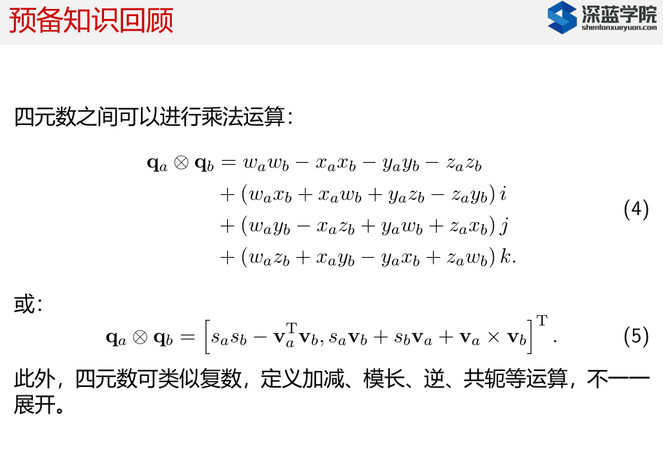
## 1.1. 四元数的基本运算 * 主要运算 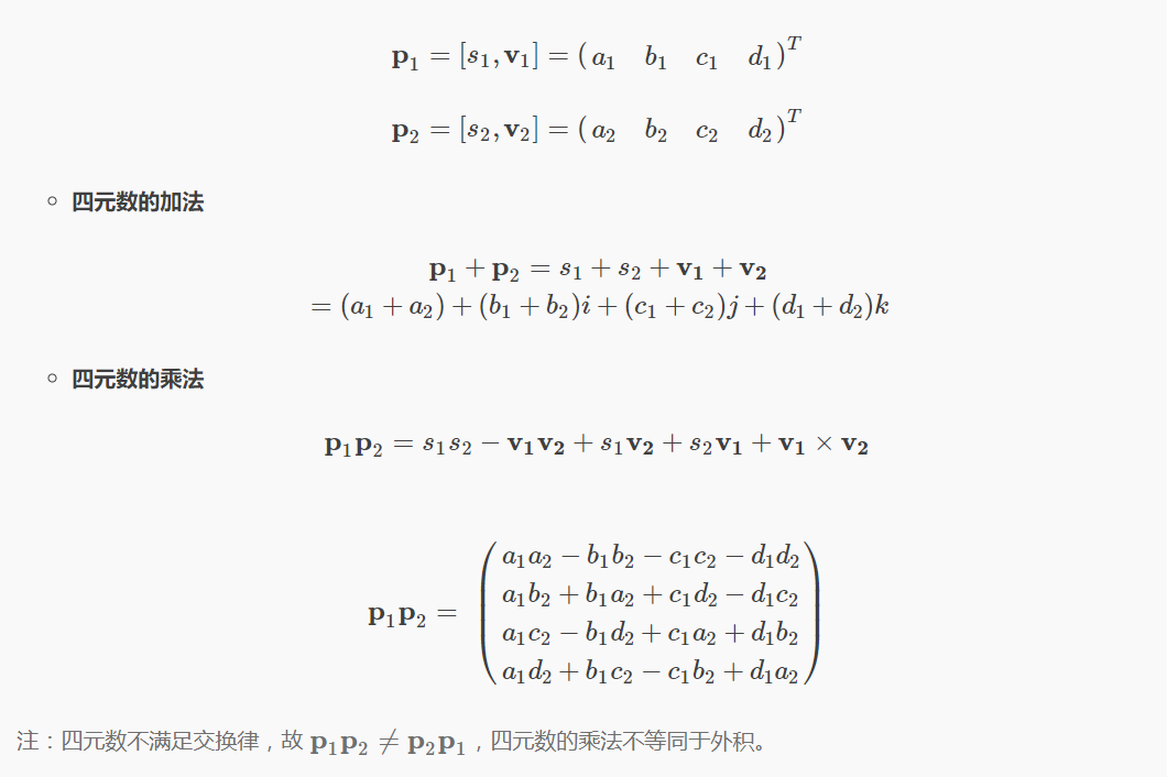 * 四元数乘法 * 四元数乘法 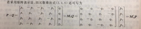 > 乘法性质 > 1. 满足结合律 > 2. 不满足交换律 > 3. 乘积的模等于模的乘积 > 4. 乘积的逆等于各个四元数的逆以相反的顺序相乘 * 其他运算 > 乘法性质 > 1. 满足结合律 > 2. 不满足交换律 > 3. 乘积的模等于模的乘积 > 4. 乘积的逆等于各个四元数的逆以相反的顺序相乘 * 其他运算 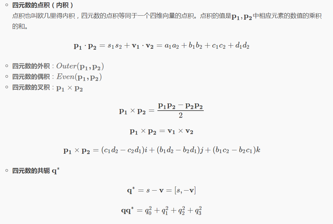 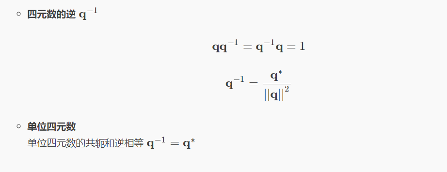 |
| *四元数部分参考:旋转矩阵、欧拉角、四元数理论及其转换关系 |
1.2. 四元数与旋转向量
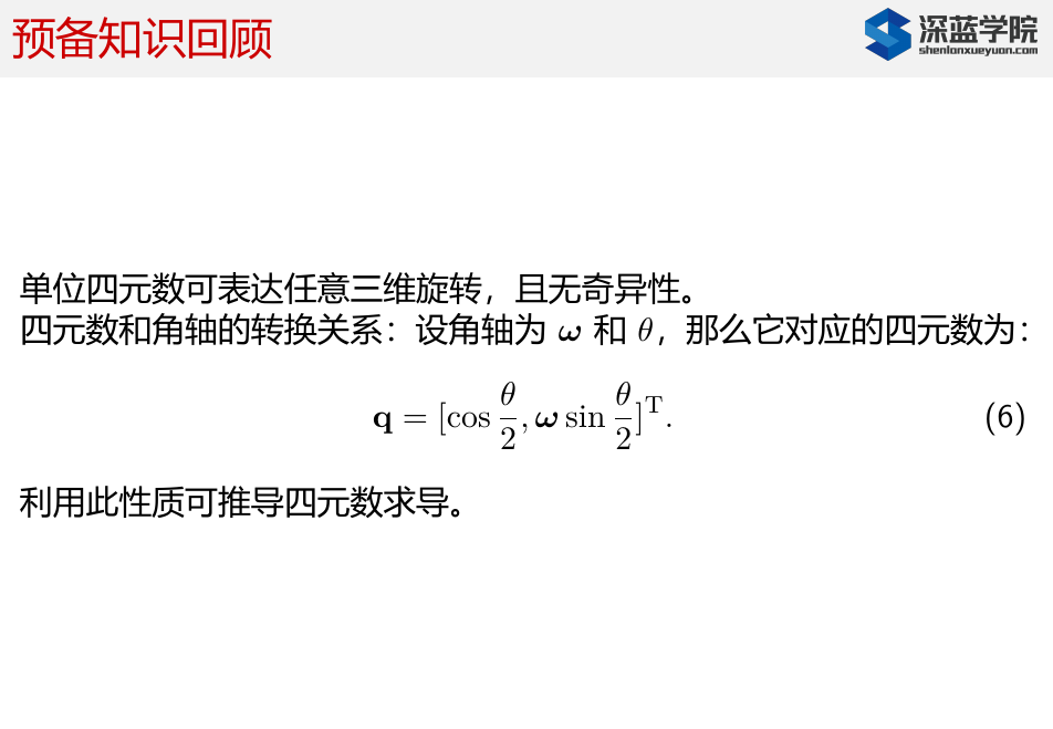 > 简单来说,四元数的思想就是把方向余弦矩阵的三次旋转表示为只绕一个旋转轴旋转一次完成,因此可以用4个数来表示这个过程,其中包括旋转轴向量的长度(θ)和旋转轴单位向量(x,y,z)
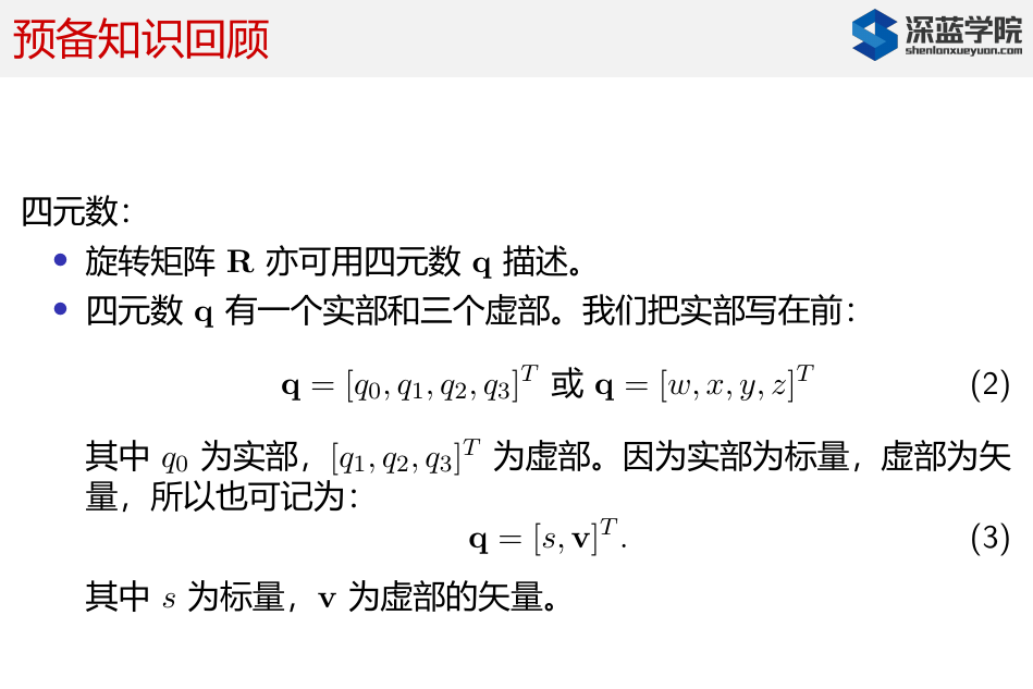
1.2.1. 四元数的表示
\[ \begin{aligned} \begin{bmatrix} q_0 \\ q_1 \\ q_2 \\ q_3 \end{bmatrix} = \begin{bmatrix} \cos \frac{\theta}{2} \\ x*\sin \frac{\theta}{2} \\ y*\sin \frac{\theta}{2} \\ z*\sin \frac{\theta}{2} \\ \end{bmatrix} \end{aligned} \]
## 1.3. 四元数对时间的导数 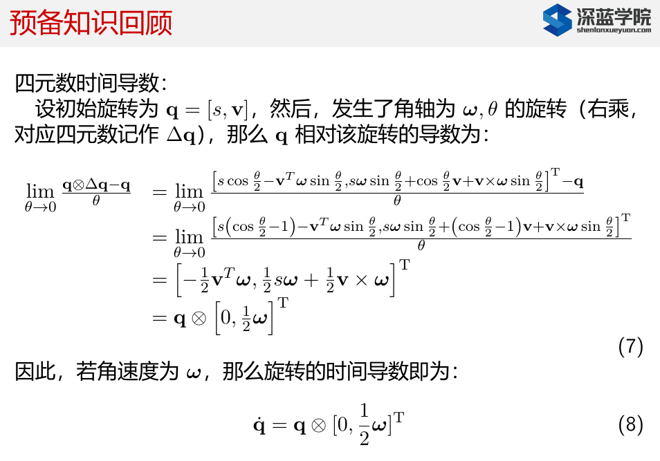 ### 1.3.1. 关于两个极限的近似(上面求极限用到的) ### 1.3.1. 关于两个极限的近似(上面求极限用到的) 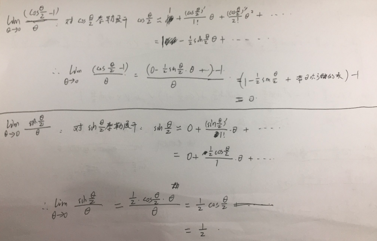 |
|---|
## 1.4. 旋转矩阵(李群SO3)对角速度\(\omega\)的求导 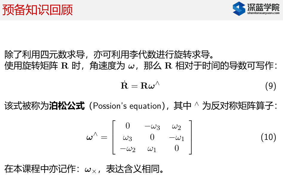 |
## 1.5. so(3) 导数 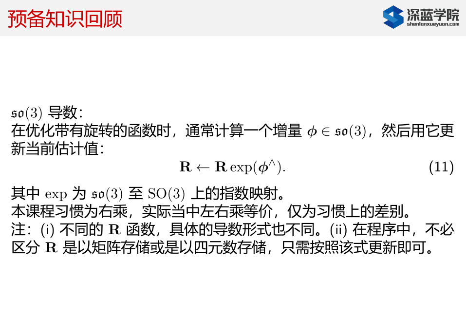 ### 1.5.1. 左乘模型 ### 1.5.1. 左乘模型 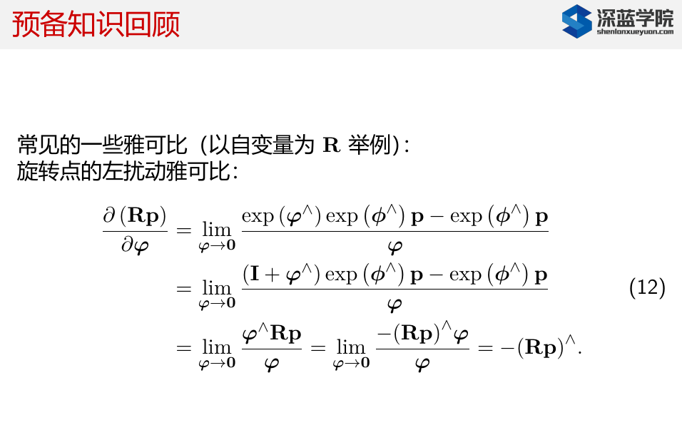 ### 1.5.2. 右乘模型 ### 1.5.2. 右乘模型 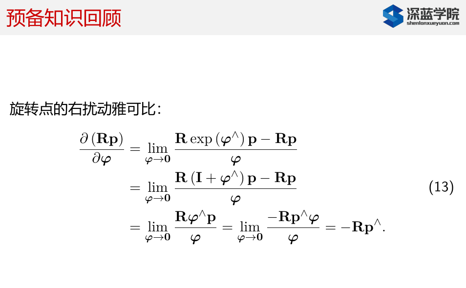 |
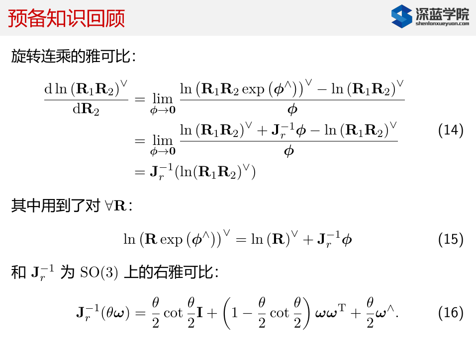
1.6. 旋转连乘的雅克比
1.6.1. 对R2求导
 ### 1.6.2. 对R1求导
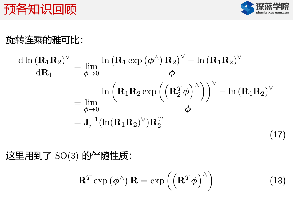
1.6.3. 伴随性质的证明
1.6.3.1. 即证明下式
\[ \begin{aligned} R~exp(\phi \hat{~} )~R^T=exp((R\phi)\hat{~}) \end{aligned} \] #### 1.6.3.2. 首先证明 \[ Rp\hat{~}R^T=(Rp)\hat{~} \] //或者:(上下是等价的) \[ \begin{aligned} R[a]_\times=[Ra]_\times R \end{aligned} \] ##### 1.6.3.2.1. 已知 若 \[ \begin{aligned} a=b\times c \end{aligned} \] 则有 \[ \begin{aligned} &R\in SO3 \\ &Ra=(Rb) \times (Rc) \end{aligned} \]
1.6.3.2.2. 可证
\[ \begin{aligned} (Rp)\hat{~}&=(Rp)\hat{~}I=(Rp)_\times RR^{T}I \\ &=(Rp)_\times (R R^{T}I) \\ &=R(p_\times R^{T}I) \\ &=Rp\hat{~}R^T \end{aligned} \]
1.6.3.3. 再来证明原式
1.6.3.3.1. 等式右侧
\[ \begin{aligned} &\because Rp\hat{~}R^T=(Rp)\hat{~} \\ &\therefore e^{(Rp)\hat{~}}=e^{Rp\hat{~}R^T} \approx I+Rp\hat{~}R^T \end{aligned} \] ##### 1.6.3.3.2. 等式左侧 \[ \begin{aligned} Re^{(p\hat{~})}R^T &\approx R(I+p\hat{~})R^T \\ &=RIR^T+Rp\hat{~}R^T \\ &=I+Rp\hat{~}R^T \end{aligned} \] ##### 1.6.3.3.3. 证毕
| ## 1.7. 不用SE3的讨论 |
 |
1.8. 作业
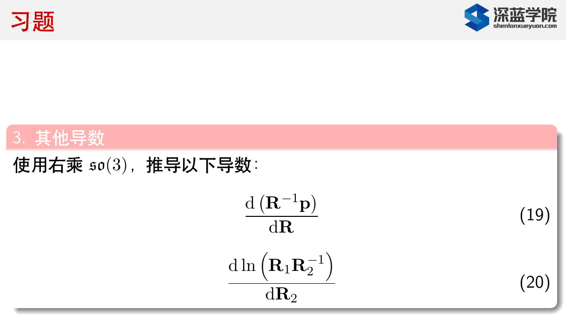
1.8.1. 使用右乘SO3,求\(\frac{d(R^{-1}p)}{dR}\)
\[ \begin{aligned} \frac{d(R^{-1}p)}{dR}&=\lim_{\phi \to 0} \frac{d[(R\exp(\phi \hat{~}))^{-1}-R^{-1}p]}{d \phi} \\ &=\lim_{\phi \to 0} \frac{d[\exp^{-1}(\phi \hat{~})~R^{-1}p-R^{-1}p]}{d \phi} \\ &=\lim_{\phi \to 0} \frac{d[\exp(-\phi \hat{~})~R^{-1}p-R^{-1}p]}{d \phi} \\ &=\lim_{\phi \to 0} \frac{d[(I-\phi \hat{~})~R^{-1}p-R^{-1}p]}{d \phi} \\ &=\lim_{\phi \to 0} \frac{-\phi\hat{~}~R^{-1}p}{\phi} \\ &=\lim_{\phi \to 0} \frac{(R^{-1}p\hat{~})\phi}{\phi} \\ &=(R^{-1}p)\hat{~} \end{aligned} \]
1.8.2. 使用右乘SO3,求\(\frac{d\ln(R_1R_2^{-1})}{dR_2}\)
\[ \begin{aligned} \frac{d\ln(R_1R_2^{-1})}{dR_2}&=\lim_{\phi \to 0} \frac{d \ln[R_1(R_2 \exp(\phi \hat{~}))^{-1}]-ln(R_1R_2^{-1})}{d \phi} \\ &=\lim_{\phi \to 0} \frac{d \ln[R_1\exp^{-1}(\phi \hat{~})R_2^{-1}]-ln(R_1R_2^{-1})}{d \phi} \\ &=\lim_{\phi \to 0} \frac{d \ln[R_1\exp(-\phi \hat{~})R_2^{-1}]-ln(R_1R_2^{-1})}{d \phi} \end{aligned} \] 再利用伴随性质 \[ \begin{aligned} R\exp(\phi \hat{~} )R^T=\exp((R\phi)\hat{~}) \end{aligned} \] 可得 \[ \begin{aligned} R_2\exp(-\phi \hat{~})R_2^T=\exp((R_2*(-\phi))\hat{~}) \end{aligned} \] 两边同时左乘\(R_2^{-1}\) \[ \begin{aligned} \exp(-\phi \hat{~})R_2^{-1}=R_2^{-1}\exp((R_2*(-\phi))\hat{~}) \end{aligned} \] 将上式带入 \[ \begin{aligned} \frac{d\ln(R_1R_2^{-1})}{dR_2}&=\lim_{\phi \to 0} \frac{d \ln[R_1(R_2 \exp(\phi \hat{~}))^{-1}]-\ln(R_1R_2^{-1})}{d \phi} \\ &=\lim_{\phi \to 0} \frac{d \ln[R_1\exp^{-1}(\phi \hat{~})R_2^{-1}]-\ln(R_1R_2^{-1})}{d \phi} \\ &=\lim_{\phi \to 0} \frac{d \ln[R_1\exp(-\phi \hat{~})R_2^{-1}]-\ln(R_1R_2^{-1})}{d \phi} \\ &=\lim_{\phi \to 0} \frac{d \ln[R_1R_2^{-1}\exp((R_2*(-\phi))\hat{~})]-\ln(R_1R_2^{-1})}{d \phi} \\ &=\lim_{\phi \to 0} \frac{d \ln(R_1R_2^{-1})+J_r^{-1}R_2*(-\phi)-\ln(R_1R_2^{-1})}{d \phi} \\ &=\lim_{\phi \to 0} \frac{d \ln(R_1R_2^{-1})-J_r^{-1}\phi R_2-\ln(R_1R_2^{-1})}{d \phi} \\ &=-J_r^{-1}(\ln(R_1R_2^{-1}))R_2 \end{aligned} \]
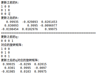
1.8.3. CODEing
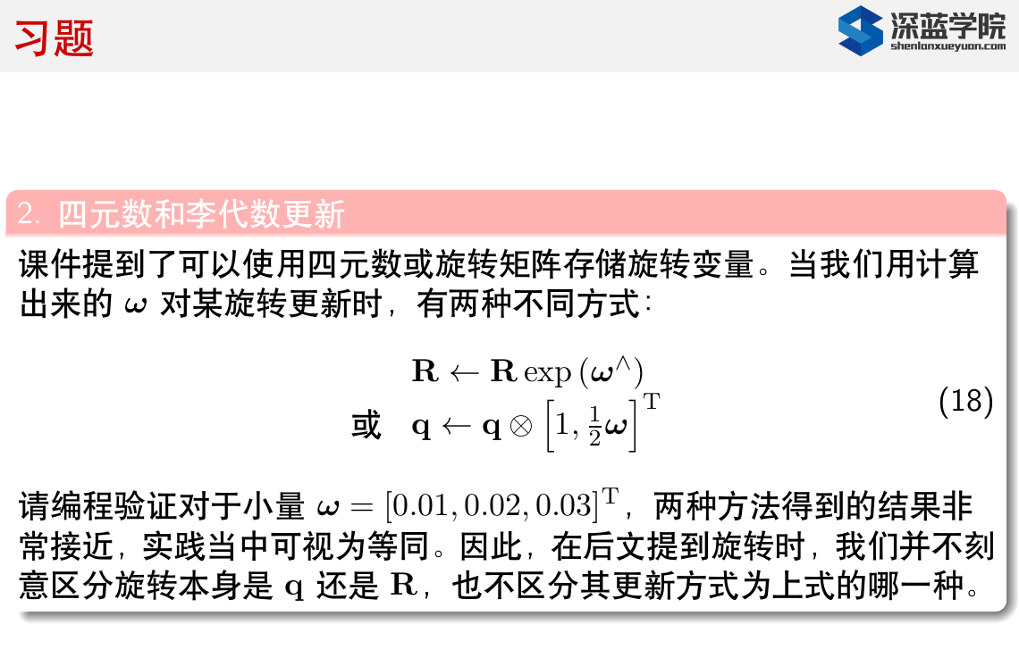
1 |
|
1.8.3.1. Result