2D-NDT-匹配算法

Catalogue
  1. 1. 正态分布变换(The Normal Distributions Transform)
    1. 1.1. 算法提出
    2. 1.2. 算法应用
    3. 1.3. 算法特点
    4. 1.4. 其他配准算法
  2. 2. 2D-NDT基本原理
    1. 2.1. 概率密度计算
    2. 2.2. 帧间配准(匹配)
    3. 2.3. 牛顿迭代法优化
  3. 3. 应用于位置跟踪
  4. 4. SLAM上的应用
    1. 4.1. 对多次扫描进行定位
    2. 4.2. 添加关键帧以及优化地图
    3. 4.3. 文章实现效果
    4. 4.4. 2020-03-06更新: PCL中关于2D-NDT的代码及注释
    5. 4.5. 参考资料

正态分布变换(The Normal Distributions Transform)

算法提出

Biber和Straer提出了二维数据配准的正态分布变换(NDT)方法。该算法中的关键元素是参考扫描的表示。不是将当前扫描直接匹配到参考扫描的点,而是通过正态分布的线性组合来模拟在特定位置找到表面点的可能性。

算法应用

  • 点云配准
  • 地图匹配

算法特点

计算正态分布是一个一次性的工作(初始化),不需要消耗大量代价计算最近邻搜索匹配点。概率密度函数在两幅图像采集之间的时间可以离线计算出来

其他配准算法

  1. ICP

    • 要剔除不合适的点对(点对距离过大、包含边界点的点对)
    • 基于点对的配准,并没有包含局部形状的信息
  2. IDC

    • ICP的一种改进,采用极坐标代替笛卡尔坐标进行最近点搜索匹配
  3. PIC

    • 考虑了点云的噪音和初始位置的不确定性
  4. Point-based probabilistic registration

  5. Gaussian fields

    • 和NDT正态分布变换类似,利用高斯混合模型考察点和点的距离和点周围表面的相似性
  6. Likelihood-field matching——随机场匹配

  7. CRF匹配

  8. Branch-and-bound registration

  9. Registration using local geometric features

2D-NDT基本原理

NDT算法论文原文是从2D角度描述的。

概率密度计算

NDT利用局部正态分布建立了一次激光扫描所有重建二维点的分布模型,首先,将机器人周围的二维空间细分为固定大小的网格(类似于占据栅格地图),然后对于每一个单元,进行下面3个操作

  • 收集在这个窗口内的所有2D点
  • 计算2D点集的质心\(q=\frac{1}{n}\sum_{i} x_i\)
  • 计算协方差矩阵\(\Sigma=\frac{1}{n}\sum_i(x_i-q)(x_i-q)^T\)

那么,在这个单元cell内观测到一个样本在该2D点\(\boldsymbol{x}=(u,v)^T\) 的概率可以用下面的正态分布来描述:

\[ \begin{aligned} p(x) \sim \exp (-\frac{(x-q)^T \Sigma^{-1}(x-q)}{2}) \end{aligned} \]

与占据栅格类似,NDT建立了平面的网格细分,但是占据栅格代表的是该栅格被占据的概率,而NDT的栅格代表的是在一个单元(cell)内的每个位置上,观测到一个样本的概率。这个操作有什么好处?好处在于使用概率密度的形式对二维平面进行了分段连续可微的描述。

在进一步描述example之前,需要提出两点需要注意的地方

  • 为了最小化离散化的影响,我们决定使用四个重叠的网格,首先放置一个边长为l的单网格,第二个则水平平移\(\frac{l}{2}\)长度,第三个则垂直方向平移\(\frac{l}{2}\)长度,而最后一个则水平和垂直都平移\(\frac{l}{2}\)长度。如下图所示,现在每个2D点都落入到这4个cell里面,因此,如果计算一个点的概率密度,即对所有四个单元的密度进行评估,并对结果进行求和。但是在下面的讨论中,暂时不考虑这样的情况,只需考虑只有1个cell即可。

  • 另外一个点就是,如果在一个完全没有噪声的理想情况下,协方差矩阵会变成奇异的,无法求逆。在实际情况中,协方差矩阵有时候十分接近奇异,为了避免这种情况,进行检查,检查协方差矩阵的最小特征值是否至少是最大特征值的0.001倍,如果不是,则设置该值。

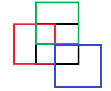
下图1展示了对激光扫描进行NDT之后的结果:

右图是NDT结果,这是通过计算每个点的概率密度得到的,高亮的部分表示着该处有较大的概率密度。接下来讨论这个变换怎么发挥作用在匹配中。

帧间配准(匹配)

给定两个机器人坐标系之间的空间映射T, \[ \begin{aligned} T= \begin{pmatrix} x' \\ y' \end{pmatrix} = \begin{pmatrix} \cos \phi & -\sin \phi \\ \sin \phi & \cos \phi \end{pmatrix} \begin{pmatrix} x \\ y \end{pmatrix} + \begin{pmatrix} t_x \\ t_y \end{pmatrix} \end{aligned} \]

其中,\((t_x,t_y)^T\)表示平移,\(\phi\)表示旋转——(两帧之间),帧间匹配就是要求出平移和旋转的量。

本文提出的基本流程是:

  1. 对第一帧进行NDT处理
  2. 参数(R,t)初始化,可设置为0或者使用里程计的数据
  3. 对于第二帧的每一个样本,利用待优化参数将第二帧的点反投影到第一帧的坐标系中
  4. 确定每个映射点对应的正态分布 ?
  5. 参数(R,t)的得分是通过评估每个映射点的分布并对结果求和来确定的
  6. 计算一个新的参数估计试图优化评分。这是通过执行牛顿算法的一个步骤完成的
  7. 重复,直到收敛

前4步就是前文所说的计算NDT变换,接下来详细介绍剩下的步骤

参数约定:

  • 待优化参数\(\boldsymbol{T}()=\boldsymbol{P}=(p_i){i=1,2,3}=(t_x,t_y,\phi)^T\)
  • 第二帧的第i个扫描点\(x_i\)
  • 第二帧的第i个扫描点反投影回第一帧坐标系后得到的点\(x_i'=T(x_i,\boldsymbol{P})\)
  • \(\Sigma_i,q_i\)分别是第二帧反投影点\(x_i'\)的联合高斯分布的协方差矩阵和均值,在第一帧的NDT变换中查找

评分函数

\[ score(p)=\sum_i \exp ( \frac{-(x_i'-q_i)^T \Sigma_i^{-1}(x_i'-q_i)}{2}) \]

这个其实就是联合高斯分布的表达,其中\(\Sigma_i^{-1}\)就是信息矩阵,也就是协方差矩阵的逆

牛顿迭代法优化

由于优化问题通常被描述为最小化问题,我们将采用这个约定的符号。最优化可以表示为最小化\(-socre\)。牛顿迭代法可以表示为求解增量方程

\[ \boldsymbol{H\Delta p}=-\boldsymbol{g} \]

其中,

  • \(\boldsymbol{g}\)是函数\(f()\)的梯度转置,也就是雅克比
  • \(\boldsymbol{H}\)是对应的海森矩阵

这个方程的解是一个增量\(\Delta p\),用来更新估计值:

\[ \boldsymbol{p} \leftarrow \boldsymbol{p} +\Delta \boldsymbol{p} \]

如果矩阵\(H\)是正定的,那么\(f(\boldsymbol{p})\)将会在增量\(\Delta \boldsymbol{p}\)的方向减小,否则使用\(\boldsymbol{H}'=\boldsymbol{H}+\lambda I\)来代替\(\boldsymbol{H}\),其中\(\lambda\)用来使得矩阵\(\boldsymbol{H}\)变成正定。

这个算法使用函数\(-score\),通过收集方程3中所有和的偏导数来建立梯度和海森矩阵。

下面的\(x_i\)将表示第i帧的点集,不再是第i个点

于是,有 \[ q=x_i'-q_i \]

所以,优化的目标函数可以写成

\[ -score= s =- \exp \frac{- \boldsymbol{q^T} \Sigma^{-1} \boldsymbol{q} }{2} \]

于是,目标函数对优化变量的梯度为

\[ \begin{aligned} \bar{g_i} &= - \frac{ \partial s}{ \partial p[i]}= - \frac{ \partial s}{ \partial q} \frac{q}{p[i]} \\ &= \boldsymbol{q^T} \Sigma^{-1} \frac{ \partial q}{ \partial p[i]} \exp \frac{- \boldsymbol{q^T} \Sigma^{-1}q}{2} \end{aligned} \]

根据变换等式2,使用线性化的来表示,有

\[ \begin{aligned} u' = \cos (p[3]) u -\sin(p[3]) v+ p[1]\\ v' = \sin (p[3]) u -\cos(p[3]) v + p[2] \end{aligned} \]

对应的雅克比可写成

\[ \begin{aligned} \boldsymbol{J_T}= \frac{\partial \boldsymbol{q} }{\partial \boldsymbol{T} }=\frac{\partial \boldsymbol{q} }{\partial \boldsymbol{P} }= \begin{pmatrix} 1 & 0 & -x \sin \phi -y \cos \phi \\ 0 & 1 & x \cos \phi - y \sin \phi \end{pmatrix} \end{aligned} \]

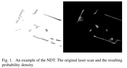
海森矩阵\(\boldsymbol{H}\):

其中,投影后的去质心点集\(\boldsymbol{q}\)对变换\(p[i],p[j]\)的二阶导\(\frac{\partial ^2 \boldsymbol{q} }{ \partial p[i] \partial p[j]}\)可以如下表示:

\[ \frac{ \partial ^2 \boldsymbol{q} }{ \partial p_i \partial p_j}= \left \{ \begin{aligned} \begin{pmatrix} -x \cos \phi + y \sin \phi \\ -x \sin \phi - y \cos \phi \end{pmatrix} ~~ i=j=3 \\ \begin{pmatrix} 0 \\ 0 \end{pmatrix} ~~~~~~~~~~~~~~~ otherwise \end{aligned} \right. \]

注意:上面的\(p[i],p[j]\)都是指同一个变换\(P\)里面的某个元素\(t_x,t_y, \phi\)其中一个。

从这些方程可以看出,建立梯度和海森矩阵的计算成本较低,每点只有一次对指数函数的调用和少量的乘法。三角函数计算仅与估计的角度\(\phi\)有关,因此每次迭代都需要计算一次。

应用于位置跟踪

下面把参考的激光扫描称为关键帧,在时间\(t=t_k\),算法执行一下流程

  • 设置一个从\(t_k-1\)\(t_k\)的运动估计作为初值\(\delta\)
  • 将当前帧的激光扫描点根据这个\(\delta\)反投影到上一个时刻的机器人坐标系下
  • 使用当前帧的扫描、参考关键帧的NDT以及新的运动估计\(\delta\)来实现优化迭代
  • 检查参考关键帧与当前帧是否比较靠近,如果是,则继续迭代,否则,采用上一次成功匹配的激光扫描作为新的关键帧。

判断一个扫描是否仍然足够近是基于一个简单的经验标准,涉及到关键帧和当前帧之间的平移和角距离以及最终的评分.

SLAM上的应用

定义地图就是对关键帧的采集以及各个关键帧的位姿。

对多次扫描进行定位

对于地图上的每帧的扫描\(i\),都拥有其位姿,位姿指该帧在全局坐标系下的,当前机器人姿态由旋转矩阵R和平移向量t表示

添加关键帧以及优化地图

地图是由一些关键帧以及它们的全局坐标系位姿组成的,如果当前扫描与地图的重叠太小,那么只取到最后一次成功匹配的扫描来组成地图。然后,每个重叠的扫描分别匹配到新的关键帧,产生两个扫描之间的相对位姿,这意味着需要维护一个图,其中包含成对匹配结果的信息。

在这个图里面,每个关键帧都使用一个节点来代表,每个节点维护着对应关键帧的世界坐标系的位姿。两个节点之间的边表示对应的扫描已经成对匹配,并维护着两个扫描之间的相对位姿,作为优化的约束条件

当一个新的关键帧插入,地图会通过优化损失函数来调整所有关键帧的位姿来进行调整。关键帧之间两两配准的结果被用来定义每一对匹配的二次误差模型如下:两次扫描的全局位姿参数可用来表示两次扫描之间的相对位姿。

如果使用\(\Delta T\)来表示(使用两次扫描的全局位姿所构成的相对位姿)与(使用NDT匹配算法得到的相对位姿)之间的,那么评分模型可以使用下面来描述

\[ socre'(\Delta T)= score + \frac{1}{2} (\Delta T)^T H (\Delta T) \]

这种全局优化的做法,当关键帧的数量变得很大的时候,难以再实时进行,因为待优化的参数随关键帧呈线性增长\(3N-3\),每个关键帧都需要3个参数,后面减3是因为第一个关键帧的位姿固定为(0,0,0),为了减少在零空间的漂移,采用固定第一帧的做法。

为了避免这个问题,文章采用使用局部图的思想,只对一个局部地图进行优化,这个局部子图通过遍历所有的关键帧,只有与当前帧相连不超过3条边的,才参与组成这个局部子图。我们现在只针对参数优化上面的错误函数,这些参数属于这个子图中包含的关键帧。

当然,如果如果要形成回环,我们将不得不优化所有关键帧。
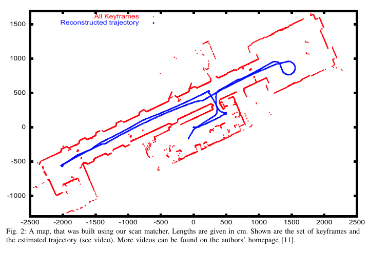
文章实现效果

2020-03-06更新: PCL中关于2D-NDT的代码及注释

PCL代码基本与论文一致

ndt_2d.h

1
2
3
4
5
6
7
8
9
10
11
12
13
14
15
16
17
18
19
20
21
22
23
24
25
26
27
28
29
30
31
32
33
34
35
36
37
38
39
40
41
42
43
44
45
46
47
48
49
50
51
52
53
54
55
56
57
58
59
60
61
62
63
64
65
66
67
68
69
70
71
72
73
74
75
76
77
78
79
80
81
82
83
84
85
86
87
88
89
90
91
92
93
94
95
96
97
98
99
100
101
102
103
104
105
106
107
108
109
110
111
112
113
114
115
116
117
118
119
120
121
122
123
#pragma once

#include <pcl/pcl_macros.h>
#include <pcl/registration/registration.h>

namespace pcl
{
/** \brief @b NormalDistributionsTransform2D provides an implementation of the
* Normal Distributions Transform algorithm for scan matching.
*
* This implementation is intended to match the definition:
* Peter Biber and Wolfgang Straßer. The normal distributions transform: A
* new approach to laser scan matching. In Proceedings of the IEEE In-
* ternational Conference on Intelligent Robots and Systems (IROS), pages
* 2743–2748, Las Vegas, USA, October 2003.
*
* \author James Crosby
*/
// 2D-NDT点云配准
template <typename PointSource, typename PointTarget>
class NormalDistributionsTransform2D : public Registration<PointSource, PointTarget>
{
using PointCloudSource = typename Registration<PointSource, PointTarget>::PointCloudSource;
using PointCloudSourcePtr = typename PointCloudSource::Ptr;
using PointCloudSourceConstPtr = typename PointCloudSource::ConstPtr;

using PointCloudTarget = typename Registration<PointSource, PointTarget>::PointCloudTarget;

using PointIndicesPtr = PointIndices::Ptr;
using PointIndicesConstPtr = PointIndices::ConstPtr;

public:

using Ptr = shared_ptr< NormalDistributionsTransform2D<PointSource, PointTarget> >;
using ConstPtr = shared_ptr< const NormalDistributionsTransform2D<PointSource, PointTarget> >;

/** \brief Empty constructor. */
// 空的构造函数
NormalDistributionsTransform2D ()
: Registration<PointSource,PointTarget> (),
grid_centre_ (0,0), grid_step_ (1,1), grid_extent_ (20,20), newton_lambda_ (1,1,1)
{
reg_name_ = "NormalDistributionsTransform2D";
}

/** \brief Empty destructor */
~NormalDistributionsTransform2D () {}

/** \brief centre of the ndt grid (target coordinate system)
* \param centre value to set
*/
// 设置NDT网格中心, 目标坐标系的, (也就是要将点云匹配过去的坐标系)
virtual void
setGridCentre (const Eigen::Vector2f& centre) { grid_centre_ = centre; }

/** \brief Grid spacing (step) of the NDT grid
* \param[in] step value to set
*/
// 步长设置
virtual void
setGridStep (const Eigen::Vector2f& step) { grid_step_ = step; }

/** \brief NDT Grid extent (in either direction from the grid centre)
* \param[in] extent value to set
*/
// 从网格中心扩展多少,也就是NDT cell范围?
virtual void
setGridExtent (const Eigen::Vector2f& extent) { grid_extent_ = extent; }

/** \brief NDT Newton optimisation step size parameter
* \param[in] lambda step size: 1 is simple newton optimisation, smaller values may improve convergence
*/
// 设置优化步长, 1是简单的牛顿迭代, 更小的值可以提高收敛效果
virtual void
setOptimizationStepSize (const double& lambda) { newton_lambda_ = Eigen::Vector3d (lambda, lambda, lambda); }

/** \brief NDT Newton optimisation step size parameter
* \param[in] lambda step size: (1,1,1) is simple newton optimisation,
* smaller values may improve convergence, or elements may be set to
* zero to prevent optimisation over some parameters
*
* This overload allows control of updates to the individual (x, y,
* theta) free parameters in the optimisation. If, for example, theta is
* believed to be close to the correct value a small value of lambda[2]
* should be used.
*/
// 重载函数, 就是说,当认为优化的时候某个变量如朝向角已经足够精确了,那么可以把 lambda[2]设置为一个小值,加快速度
virtual void
setOptimizationStepSize (const Eigen::Vector3d& lambda) { newton_lambda_ = lambda; }

protected:
/** \brief Rigid transformation computation method with initial guess.
* \param[out] output the transformed input point cloud dataset using the rigid transformation found
* \param[in] guess the initial guess of the transformation to compute
*/
// 使用初始位姿计算点云之间的变换矩阵,输出: 利用变换将输入点云匹配到目标点云
void
computeTransformation (PointCloudSource &output, const Eigen::Matrix4f &guess) override;

using Registration<PointSource, PointTarget>::reg_name_;
using Registration<PointSource, PointTarget>::target_;
using Registration<PointSource, PointTarget>::converged_;
using Registration<PointSource, PointTarget>::nr_iterations_;
using Registration<PointSource, PointTarget>::max_iterations_;
using Registration<PointSource, PointTarget>::transformation_epsilon_;
using Registration<PointSource, PointTarget>::transformation_rotation_epsilon_;
using Registration<PointSource, PointTarget>::transformation_;
using Registration<PointSource, PointTarget>::previous_transformation_;
using Registration<PointSource, PointTarget>::final_transformation_;
using Registration<PointSource, PointTarget>::update_visualizer_;
using Registration<PointSource, PointTarget>::indices_;

Eigen::Vector2f grid_centre_;
Eigen::Vector2f grid_step_;
Eigen::Vector2f grid_extent_;
Eigen::Vector3d newton_lambda_;
public:
PCL_MAKE_ALIGNED_OPERATOR_NEW
};

} // namespace pcl

#include <pcl/registration/impl/ndt_2d.hpp>

ndt_2d.hpp

1
2
3
4
5
6
7
8
9
10
11
12
13
14
15
16
17
18
19
20
21
22
23
24
25
26
27
28
29
30
31
32
33
34
35
36
37
38
39
40
41
42
43
44
45
46
47
48
49
50
51
52
53
54
55
56
57
58
59
60
61
62
63
64
65
66
67
68
69
70
71
72
73
74
75
76
77
78
79
80
81
82
83
84
85
86
87
88
89
90
91
92
93
94
95
96
97
98
99
100
101
102
103
104
105
106
107
108
109
110
111
112
113
114
115
116
117
118
119
120
121
122
123
124
125
126
127
128
129
130
131
132
133
134
135
136
137
138
139
140
141
142
143
144
145
146
147
148
149
150
151
152
153
154
155
156
157
158
159
160
161
162
163
164
165
166
167
168
169
170
171
172
173
174
175
176
177
178
179
180
181
182
183
184
185
186
187
188
189
190
191
192
193
194
195
196
197
198
199
200
201
202
203
204
205
206
207
208
209
210
211
212
213
214
215
216
217
218
219
220
221
222
223
224
225
226
227
228
229
230
231
232
233
234
235
236
237
238
239
240
241
242
243
244
245
246
247
248
249
250
251
252
253
254
255
256
257
258
259
260
261
262
263
264
265
266
267
268
269
270
271
272
273
274
275
276
277
278
279
280
281
282
283
284
285
286
287
288
289
290
291
292
293
294
295
296
297
298
299
300
301
302
303
304
305
306
307
308
309
310
311
312
313
314
315
316
317
318
319
320
321
322
323
324
325
326
327
328
329
330
331
332
333
334
335
336
337
338
339
340
341
342
343
344
345
346
347
348
349
350
351
352
353
354
355
356
357
358
359
360
361
362
363
364
365
366
367
368
369
370
371
372
373
374
375
376
377
378
379
380
381
382
383
384
385
386
387
388
389
390
391
392
393
394
395
396
397
398
399
400
401
402
403
404
405
406
407
408
409
410
411
412
413
414
415
416
417
418
419
420
421
422
423
424
425
426
427
428
429
430
431
432
433
434
435
436
437
438
439
440
441
442
443
444
445
446
447
448
449
450
451
452
453
454
455
456
457
458
459
460
461
462
463
464
465
466
467
468
469
470
471
472
473
474
475
476
477
478
479
480
481
482
483
484
485
486
487
488
489
490
491
492
493
494
495
496
497
498
499
500
501
502
503
504
505
506
507
508
509
510
511
512
513
514
515
516
517
518
519
520
521
522
523
524
525
526
527
528
529
530
531
532
533
534
535
536
537
538
539
540
541
542
543
544
545
546
#ifndef PCL_NDT_2D_IMPL_H_
#define PCL_NDT_2D_IMPL_H_

#include <pcl/registration/eigen.h>
#include <pcl/registration/boost.h>

#include <cmath>
#include <memory>

namespace pcl
{
namespace ndt2d
{
/** \brief Class to store vector value and first and second derivatives
* (grad vector and hessian matrix), so they can be returned easily from
* functions
*/
// 储存一阶导数和二阶导数
// 可以看做是增量方程
template<unsigned N=3, typename T=double>
struct ValueAndDerivatives
{
ValueAndDerivatives () : hessian (), grad (), value () {}

Eigen::Matrix<T, N, N> hessian;
Eigen::Matrix<T, N, 1> grad;
T value;

static ValueAndDerivatives<N,T>
Zero ()
{
ValueAndDerivatives<N,T> r;
r.hessian = Eigen::Matrix<T, N, N>::Zero ();
r.grad = Eigen::Matrix<T, N, 1>::Zero ();
r.value = 0;
return r;
}

ValueAndDerivatives<N,T>&
operator+= (ValueAndDerivatives<N,T> const& r)
{
hessian += r.hessian;
grad += r.grad;
value += r.value;
return *this;
}
};

/** \brief A normal distribution estimation class.
*
* First the indices of of the points from a point cloud that should be
* modelled by the distribution are added with addIdx (...).
*
* Then estimateParams (...) uses the stored point indices to estimate the
* parameters of a normal distribution, and discards the stored indices.
*
* Finally the distriubution, and its derivatives, may be evaluated at any
* point using test (...).
*/
// 这是单个cell的NDT模型
// 可以理解为某个cell
template <typename PointT>
class NormalDist
{
using PointCloud = pcl::PointCloud<PointT>;

public:
NormalDist ()
: min_n_ (3), n_ (0)
{
}

/** \brief Store a point index to use later for estimating distribution parameters.
* \param[in] i Point index to store
*/
void
addIdx (std::size_t i)
{
pt_indices_.push_back (i);
}

/** \brief Estimate the normal distribution parameters given the point indices provided. Memory of point indices is cleared.
* \param[in] cloud Point cloud corresponding to indices passed to addIdx.
* \param[in] min_covar_eigvalue_mult Set the smallest eigenvalue to this times the largest.
*/
// 给定cell网格中的点云,估计正态分布参数 (主要是均值和方差)
void
estimateParams (const PointCloud& cloud, double min_covar_eigvalue_mult = 0.001)
{
Eigen::Vector2d sx = Eigen::Vector2d::Zero ();
Eigen::Matrix2d sxx = Eigen::Matrix2d::Zero ();

// sx: 对所有点的x,y分别求和
// sxx: 2维向量,分别是 点云的 x^2和, y^2和
for (auto i = pt_indices_.cbegin (); i != pt_indices_.cend (); i++)
{
Eigen::Vector2d p (cloud[*i]. x, cloud[*i]. y);
sx += p;
sxx += p * p.transpose ();
}

n_ = pt_indices_.size ();

// 检查cell网格中的点云里面点的个数是否大于3
if (n_ >= min_n_)
{
// 求质心,存到mean_
mean_ = sx / static_cast<double> (n_);
// Using maximum likelihood estimation as in the original paper
// 计算协方差矩阵
Eigen::Matrix2d covar = (sxx - 2 * (sx * mean_.transpose ())) / static_cast<double> (n_) + mean_ * mean_.transpose ();

// 求特征值
Eigen::SelfAdjointEigenSolver<Eigen::Matrix2d> solver (covar);
// 如果最小的特征值比 0.001*最大的特征值小,则不需要修正协方差矩阵
if (solver.eigenvalues ()[0] < min_covar_eigvalue_mult * solver.eigenvalues ()[1])
{
// 否则,修正协方差矩阵,
PCL_DEBUG ("[pcl::NormalDist::estimateParams] NDT normal fit: adjusting eigenvalue %f\n", solver.eigenvalues ()[0]);
Eigen::Matrix2d l = solver.eigenvalues ().asDiagonal ();
Eigen::Matrix2d q = solver.eigenvectors ();
// set minimum smallest eigenvalue:
// 将最小的特征值设置为最大特征值的0.0001倍
l (0,0) = l (1,1) * min_covar_eigvalue_mult;
// 重新合成协方差矩阵
covar = q * l * q.transpose ();
}
// 储存协方差矩阵的逆,即信息矩阵
covar_inv_ = covar.inverse ();
}
// 清空点云
pt_indices_.clear ();
}

/** \brief Return the 'score' (denormalised likelihood) and derivatives of score of the point p given this distribution.
* \param[in] transformed_pt Location to evaluate at.
* \param[in] cos_theta sin(theta) of the current rotation angle of rigid transformation: to avoid repeated evaluation
* \param[in] sin_theta cos(theta) of the current rotation angle of rigid transformation: to avoid repeated evaluation
* estimateParams must have been called after at least three points were provided, or this will return zero.
*
*/
// 输入 要变换的点pt, 旋转变换的 cos,sin
// estimateParams必须在至少提供了三个点之后调用,否则将返回零
ValueAndDerivatives<3,double>
test (const PointT& transformed_pt, const double& cos_theta, const double& sin_theta) const
{
// 如果输入的点云数<3,则返回 导数为0
if (n_ < min_n_)
return ValueAndDerivatives<3,double>::Zero ();

// 开始计算导数
ValueAndDerivatives<3,double> r;
// 取变换之后的点
const double x = transformed_pt.x;
const double y = transformed_pt.y;
const Eigen::Vector2d p_xy (transformed_pt.x, transformed_pt.y);
// 该点减去目标点云的质心
const Eigen::Vector2d q = p_xy - mean_;
// 求出将该点坐标代入 NDT 分布之后得到的值 exp(-0.5*[q.transpose () * covar_inv_*q])
const Eigen::RowVector2d qt_cvi (q.transpose () * covar_inv_); // 转成行向量1x2
const double exp_qt_cvi_q = std::exp (-0.5 * double (qt_cvi * q));
// 这是增量方程等式的右侧,即b
r.value = -exp_qt_cvi_q;

// 下面开始求雅克比
// 与论文一一对应
Eigen::Matrix<double, 2, 3> jacobian;
jacobian <<
1, 0, -(x * sin_theta + y*cos_theta),
0, 1, x * cos_theta - y*sin_theta;

// 储存梯度
for (std::size_t i = 0; i < 3; i++)
r.grad[i] = double (qt_cvi * jacobian.col (i)) * exp_qt_cvi_q;

// second derivative only for i == j == 2:
// 下面求海森矩阵, 只有在i=j=2的时候才有二阶导
const Eigen::Vector2d d2q_didj (
y * sin_theta - x*cos_theta,
-(x * sin_theta + y*cos_theta)
);

for (std::size_t i = 0; i < 3; i++)
for (std::size_t j = 0; j < 3; j++)
r.hessian (i,j) = -exp_qt_cvi_q * (
double (-qt_cvi*jacobian.col (i)) * double (-qt_cvi*jacobian.col (j)) +
(-qt_cvi * ((i==2 && j==2)? d2q_didj : Eigen::Vector2d::Zero ())) +
(-jacobian.col (j).transpose () * covar_inv_ * jacobian.col (i))
);

//返回与增量方程相关的参数 r
return r;
}

protected:
const std::size_t min_n_;

std::size_t n_;
std::vector<std::size_t> pt_indices_;
Eigen::Vector2d mean_;
Eigen::Matrix2d covar_inv_;
};

/** \brief Build a set of normal distributions modelling a 2D point cloud,
* and provide the value and derivatives of the model at any point via the
* test (...) function.
*/
// 一个点云中的NDT模型的集合(每个cell都有一个NDT)
template <typename PointT>
class NDTSingleGrid: public boost::noncopyable
{
using PointCloud = pcl::PointCloud<PointT>;
using PointCloudConstPtr = typename PointCloud::ConstPtr;
using NormalDist = pcl::ndt2d::NormalDist<PointT>; // 一个cell

public:
// 构造
NDTSingleGrid (PointCloudConstPtr cloud,
const Eigen::Vector2f& about,
const Eigen::Vector2f& extent,
const Eigen::Vector2f& step)
: min_ (about - extent), max_ (min_ + 2*extent), step_ (step),
cells_ ((max_[0]-min_[0]) / step_[0],
(max_[1]-min_[1]) / step_[1]),
normal_distributions_ (cells_[0], cells_[1])
{
// about : 给定点云中,准备建立的某个cell的中心点的坐标?
// extent: cell划分范围
// step : 步长?

// sort through all points, assigning them to distributions:
std::size_t used_points = 0;
// 遍历点云里面的所有点
for (std::size_t i = 0; i < cloud->size (); i++)
if (NormalDist* n = normalDistForPoint (cloud->at (i))) // 计算点P落在哪一个cell
{
//n : 某个cell
//向该cell添加这个点在总点云的索引i
n->addIdx (i);
used_points++;
}

PCL_DEBUG ("[pcl::NDTSingleGrid] NDT single grid %dx%d using %d/%d points\n", cells_[0], cells_[1], used_points, cloud->size ());

// then bake the distributions such that they approximate the
// points (and throw away memory of the points)
// 将点云中每个点都分配到各个cell之后,对各个cell进行参数计算
for (int x = 0; x < cells_[0]; x++)
for (int y = 0; y < cells_[1]; y++)
normal_distributions_.coeffRef (x,y).estimateParams (*cloud);
}

/** \brief Return the 'score' (denormalised likelihood) and derivatives of score of the point p given this distribution.
* \param[in] transformed_pt Location to evaluate at.
* \param[in] cos_theta sin(theta) of the current rotation angle of rigid transformation: to avoid repeated evaluation
* \param[in] sin_theta cos(theta) of the current rotation angle of rigid transformation: to avoid repeated evaluation
*/
ValueAndDerivatives<3,double>
test (const PointT& transformed_pt, const double& cos_theta, const double& sin_theta) const
{
// 输入某个变换之后的点,以及cos ,sin
// 得到变换之后的点所对应的cell对象
const NormalDist* n = normalDistForPoint (transformed_pt);
// index is in grid, return score from the normal distribution from
// the correct part of the grid:
// 如果该点在范围内,即对应的cell对象存在
if (n)
return n->test (transformed_pt, cos_theta, sin_theta); //根据参数计算并返回该cell的增量方程
return ValueAndDerivatives<3,double>::Zero ();
}

protected:
/** \brief Return the normal distribution covering the location of point p
* \param[in] p a point
*/
// 这个函数输入点云中的一个点P,根据窗口范围、步长等参数,计算该点P落在哪一个cell
// 然后返回那个cell的对象
NormalDist*
normalDistForPoint (PointT const& p) const
{
// this would be neater in 3d...
// 计算该3D点应该落在哪个cell?
Eigen::Vector2f idxf;
for (std::size_t i = 0; i < 2; i++)
idxf[i] = (p.getVector3fMap ()[i] - min_[i]) / step_[i]; //idxf[]:储存对应cell的行号,列号
// 检查该点是否落在总的划分范围内
Eigen::Vector2i idxi = idxf.cast<int> ();
for (std::size_t i = 0; i < 2; i++)
if (idxi[i] >= cells_[i] || idxi[i] < 0)
return nullptr;

//
// const cast to avoid duplicating this function in const and
// non-const variants...
// 返回类型为NormalDist的东西,就是某个cell,
return const_cast<NormalDist*> (&normal_distributions_.coeffRef (idxi[0], idxi[1]));
}

Eigen::Vector2f min_;
Eigen::Vector2f max_;
Eigen::Vector2f step_;
Eigen::Vector2i cells_; // 将原始点云分割的网格数, []

//这个Matrix[i][j]表示将点云划分之后的 第i行第j列的cell
//使用Eigen::Matrix 来储存 cell对象?
Eigen::Matrix<NormalDist, Eigen::Dynamic, Eigen::Dynamic> normal_distributions_;
};

/** \brief Build a Normal Distributions Transform of a 2D point cloud. This
* consists of the sum of four overlapping models of the original points
* with normal distributions.
* The value and derivatives of the model at any point can be evaluated
* with the test (...) function.
*/
// 建立一个二维点云的正态分布变换(这是4个NDT模型的叠加)
// 这个是由四个重叠的模型组成的,每个模型有各自的原始点与正态分布
// 一些值以及微分项由test函数计算
template <typename PointT>
class NDT2D: public boost::noncopyable
{
using PointCloud = pcl::PointCloud<PointT>;
using PointCloudConstPtr = typename PointCloud::ConstPtr;
// 点云的{所有cell的集合}(储存着每个cell的NDT模型)
// 一个NDTSingleGrid对应着总点云的中心、窗口大小、步长等参数
// 下面会使用4个不同的中心,得到同一个总点云的4组{cell集合}
using SingleGrid = NDTSingleGrid<PointT>;

public:
/** \brief
* \param[in] cloud the input point cloud
* \param[in] about Centre of the grid for normal distributions model
* \param[in] extent Extent of grid for normal distributions model
* \param[in] step Size of region that each normal distribution will model
*/
// 输入原始点云,中心,范围,步长
NDT2D (PointCloudConstPtr cloud,
const Eigen::Vector2f& about,
const Eigen::Vector2f& extent,
const Eigen::Vector2f& step)
{
Eigen::Vector2f dx (step[0]/2, 0);
Eigen::Vector2f dy (0, step[1]/2);
//以窗口为中心,得到中心点进行偏移之后的cell集合, 一共得到4组cell集合
single_grids_[0].reset(new SingleGrid (cloud, about, extent, step));
single_grids_[1].reset(new SingleGrid (cloud, about +dx, extent, step));
single_grids_[2].reset(new SingleGrid (cloud, about +dy, extent, step));
single_grids_[3].reset(new SingleGrid (cloud, about +dx+dy, extent, step));
}

/** \brief Return the 'score' (denormalised likelihood) and derivatives of score of the point p given this distribution.
* \param[in] transformed_pt Location to evaluate at.
* \param[in] cos_theta sin(theta) of the current rotation angle of rigid transformation: to avoid repeated evaluation
* \param[in] sin_theta cos(theta) of the current rotation angle of rigid transformation: to avoid repeated evaluation
*/
ValueAndDerivatives<3,double>
test (const PointT& transformed_pt, const double& cos_theta, const double& sin_theta) const
{
// 输入某个来自当前帧的点P利用变换矩阵转换之后的投影点Pt,以及转换参数 cos , sin
// 计算4组cell集合各自的增量方程,然后求和,得到一个新的增量方程,也就是最终的增量方程
ValueAndDerivatives<3,double> r = ValueAndDerivatives<3,double>::Zero ();
for (const auto &single_grid : single_grids_)
r += single_grid->test (transformed_pt, cos_theta, sin_theta);
return r;
}

protected:
std::shared_ptr<SingleGrid> single_grids_[4];
};

} // namespace ndt2d
} // namespace pcl


namespace Eigen
{
/* This NumTraits specialisation is necessary because NormalDist is used as
* the element type of an Eigen Matrix.
*/
template<typename PointT> struct NumTraits<pcl::ndt2d::NormalDist<PointT> >
{
using Real = double;
using Literal = double;
static Real dummy_precision () { return 1.0; }
enum {
IsComplex = 0,
IsInteger = 0,
IsSigned = 0,
RequireInitialization = 1,
ReadCost = 1,
AddCost = 1,
MulCost = 1
};
};
}

//////////////////////////////////////////////////////////////////////////////////////////////////////////////////
template <typename PointSource, typename PointTarget> void
pcl::NormalDistributionsTransform2D<PointSource, PointTarget>::computeTransformation (PointCloudSource &output, const Eigen::Matrix4f &guess)
{
// 这是要输出的点云
PointCloudSource intm_cloud = output;

nr_iterations_ = 0;
converged_ = false;

if (guess != Eigen::Matrix4f::Identity ())
{
transformation_ = guess;
transformPointCloud (output, intm_cloud, transformation_);
}

// build Normal Distribution Transform of target cloud:
// 为目标点云创建NDT变换
// target_ndt里面包含了目标点云的所有cell的NDT分布
// 后面会调用target_ndt.test()函数,通过计算点落在哪一个cell中,根据该cell的NDT分布计算出关于该点P的增量方程
ndt2d::NDT2D<PointTarget> target_ndt (target_, grid_centre_, grid_extent_, grid_step_);

// can't seem to use .block<> () member function on transformation_
// directly... gcc bug?
// 设置初始值
Eigen::Matrix4f& transformation = transformation_;


// work with x translation, y translation and z rotation: extending to 3D
// would be some tricky maths, but not impossible.
const Eigen::Matrix3f initial_rot (transformation.block<3,3> (0,0));
const Eigen::Vector3f rot_x (initial_rot*Eigen::Vector3f::UnitX ());
// y/x
const double z_rotation = std::atan2 (rot_x[1], rot_x[0]);

// 从4x4的变换矩阵T,提取2D所需的3个维度,构成3x1向量
Eigen::Vector3d xytheta_transformation (
transformation (0,3),
transformation (1,3),
z_rotation
);

// 开始迭代
while (!converged_)
{
// 利用角度yaw求 cos , sin
const double cos_theta = std::cos (xytheta_transformation[2]);
const double sin_theta = std::sin (xytheta_transformation[2]);
// 将当前变换保存
previous_transformation_ = transformation;

// ValueAndDerivatives: 储存一阶导数和二阶导数的类
ndt2d::ValueAndDerivatives<3, double> score = ndt2d::ValueAndDerivatives<3, double>::Zero ();
// 将源点云中的每个点intm_cloud[i],代入到目标点云的NDT 正太分布函数,构造增量方程,增量方程参数储存在score
for (std::size_t i = 0; i < intm_cloud.size (); i++)
score += target_ndt.test (intm_cloud[i], cos_theta, sin_theta);

PCL_DEBUG ("[pcl::NormalDistributionsTransform2D::computeTransformation] NDT score %f (x=%f,y=%f,r=%f)\n",
float (score.value), xytheta_transformation[0], xytheta_transformation[1], xytheta_transformation[2]
);

// 检查增量方程右侧是否为0
if (score.value != 0)
{
// 通过特征值分解,进行检查
// 检查系数矩阵是否正定,否则修正系数矩阵
// test for positive definiteness, and adjust to ensure it if necessary:
Eigen::EigenSolver<Eigen::Matrix3d> solver;
solver.compute (score.hessian, false);
double min_eigenvalue = 0;
for (int i = 0; i <3; i++)
if (solver.eigenvalues ()[i].real () < min_eigenvalue)
min_eigenvalue = solver.eigenvalues ()[i].real ();

// 如果最小的特征值<0,则进行修正 通过加上 lambda * I 的对角矩阵
// ensure "safe" positive definiteness: this is a detail missing
// from the original paper
if (min_eigenvalue < 0)
{
double lambda = 1.1 * min_eigenvalue - 1;
score.hessian += Eigen::Vector3d (-lambda, -lambda, -lambda).asDiagonal ();
solver.compute (score.hessian, false);
PCL_DEBUG ("[pcl::NormalDistributionsTransform2D::computeTransformation] adjust hessian: %f: new eigenvalues:%f %f %f\n",
float (lambda),
solver.eigenvalues ()[0].real (),
solver.eigenvalues ()[1].real (),
solver.eigenvalues ()[2].real ()
);
}
// 异常检查
assert (solver.eigenvalues ()[0].real () >= 0 &&
solver.eigenvalues ()[1].real () >= 0 &&
solver.eigenvalues ()[2].real () >= 0);

// 直接得到增量 delta_T = -H^T*J
Eigen::Vector3d delta_transformation (-score.hessian.inverse () * score.grad);
// 利用增量计算得到新的变换矩阵 T_new = T_old + lambda * delta_T
// cwiseProduct()函数允许Matrix直接进行点对点乘法
Eigen::Vector3d new_transformation = xytheta_transformation + newton_lambda_.cwiseProduct (delta_transformation);

// 输出新的变换
xytheta_transformation = new_transformation;

// update transformation matrix from x, y, theta:
// 更新变换矩阵
transformation.block<3,3> (0,0).matrix () = Eigen::Matrix3f (Eigen::AngleAxisf (static_cast<float> (xytheta_transformation[2]), Eigen::Vector3f::UnitZ ()));
transformation.block<3,1> (0,3).matrix () = Eigen::Vector3f (static_cast<float> (xytheta_transformation[0]), static_cast<float> (xytheta_transformation[1]), 0.0f);

//std::cout << "new transformation:\n" << transformation << std::endl;
}
else
{
// 如果增量方程右侧=0, 无法求解
PCL_ERROR ("[pcl::NormalDistributionsTransform2D::computeTransformation] no overlap: try increasing the size or reducing the step of the grid\n");
break;
}

// 利用这次迭代出来的变换,将当前点云 变换到 目标点云坐标系上,得到intm_cloud
transformPointCloud (output, intm_cloud, transformation);

// 迭代次数+1
nr_iterations_++;

// 更新可视化?
if (update_visualizer_)
update_visualizer_ (output, *indices_, *target_, *indices_);

//std::cout << "eps=" << std::abs ((transformation - previous_transformation_).sum ()) << std::endl;


// 检查与上一次变换的差,是否足够小,如果很小了,表示收敛,优化完成
Eigen::Matrix4f transformation_delta = transformation.inverse() * previous_transformation_;
double cos_angle = 0.5 * (transformation_delta.coeff (0, 0) + transformation_delta.coeff (1, 1) + transformation_delta.coeff (2, 2) - 1);
double translation_sqr = transformation_delta.coeff (0, 3) * transformation_delta.coeff (0, 3) +
transformation_delta.coeff (1, 3) * transformation_delta.coeff (1, 3) +
transformation_delta.coeff (2, 3) * transformation_delta.coeff (2, 3);

if (nr_iterations_ >= max_iterations_ ||
((transformation_epsilon_ > 0 && translation_sqr <= transformation_epsilon_) && (transformation_rotation_epsilon_ > 0 && cos_angle >= transformation_rotation_epsilon_)) ||
((transformation_epsilon_ <= 0) && (transformation_rotation_epsilon_ > 0 && cos_angle >= transformation_rotation_epsilon_)) ||
((transformation_epsilon_ > 0 && translation_sqr <= transformation_epsilon_) && (transformation_rotation_epsilon_ <= 0)))
{
converged_ = true;
}
}
// 输出
final_transformation_ = transformation;
output = intm_cloud;
}

#endif // PCL_NDT_2D_IMPL_H_

参考资料